Pentaho Data Integration: Designing a highly available scalable s

Pentaho Data Integration: Designing a highly available scalable solution for processing files

Tutorial Details

• Software: PDI/Kettle 4.1 (download here) and MySQL server, both installed on your PC.
• Knowledge: Intermediate (To follow this tutorial you should have good knowledge of the software and hence not every single step will be described)
  
• Files: Download from here



Preparation

Set up slave servers

On Windows

On Linux

Define Slave Servers

Monitor Slave Servers

Distribution of the workload

Test the whole process

The raw data generated each year is increasing significantly. Nowadays we are dealing with huge amounts of data that have to be processed by our ETL jobs. Pentaho Data Integration/Kettle offers quite some interesting features that allow clustered processing of data. The goal of this session is to explain how to spread the ETL workload across multiple slave servers. Matt Casters originally provided the ETL files and background knowledge. My way to thank him is to provide this documentation.

Note: This solutions runs ETL jobs on a cluster in parallel independently from each other. It's like saying: Do exactly the same thing on another server without bothering what the other jobs do on the other servers. Kettle allows a different setup as well, where ETL processes running on different servers can send i.e. the result set to a master (so that all data is combined) for sorting and further processing (We will not cover this in this session). 

Preparation

Download the accompanying files from here and extract them in a directory of your choice. Keep the folder structure as is, with the root folder named ETL. If you inspect the folders, you will see that there is:

• an input directory, which stores all the files that our ETL process has to process
• an archive directory, which will store the processed files
• a PDI directory, which holds all the Kettle transformations and jobs

Create the ETL_HOME variable in the kettle.properties file (which can be found in C:\Users\dsteiner\.kettle\kettle.properties)

ETL_HOME=C\:\\ETL

Adjust the directory path accordingly.

Navigate to the simple-jndi folder in the data-integration directory. Open jdbc.properties and add following lines at the end of the file (change if necessary):

etl/type=javax.sql.DataSource

etl/driver=com.mysql.jdbc.Driver

etl/url=jdbc:mysql://localhost/etl

etl/user=root

etl/password=root

Next, start your local MySQL server and open your favourite SQL client. Run following statement:

CREATE SCHEMA etl;

USE etl;

CREATE TABLE FILE_QUEUE

(

filename VARCHAR(256)

, assigned_slave VARCHAR(256)

, finished_status VARCHAR(20)

, queued_date DATETIME

, started_date DATETIME

, finished_date DATETIME

)

;

This table will allow us to keep track of the files that have to be processed.

Set up slave servers

For the purpose of this exercise, we keep it simple and have all slaves running on localhost. Setting up a proper cluster is out of this scope of this tutorial.

Kettle comes with a lightweight web server called Carte. All that Carte does is listen to incoming job or transformation calls and process them. For more info about Carte have a look at my Carte tutorial.

So all we have to do now is to start our Carte instances:

On Windows

On the command line, navigate to the data-integration directory within your PDI folder. Run following command:

carte.bat localhost 8081

Open a new command line window and do exactly the same, but now for port 8082. 

Do the same for port 8083 and 8084.

On Linux

Open Terminal and navigate to the data-integration directory within your PDI folder. Run following command:

sh carte.sh localhost 8081

Proceed by doing exactly the same, but now for ports 8082, 8083 and 8084.

Now that all our slave servers are running, we can have a look at the ETL process ...

Populate File Queue

Start Kettle (spoon.bat or spoon.sh) and open Populate file queue.ktr (You can find it in the /ETL/PDI folder). If you have Kettle (Spoon) already running, restart it so that the changes can take effect and then open the file.

This transformation will get all filenames from the input directory (of the files that haven't been processed yet) and stores them in the FILE_QUEUE table. 

Double click on the Get file names step and click Show filename(s) … . This should show all your file names properly:

Click Close and then OK.

Next, double click on the Lookup entry in FILE_QUEUE step. Click on Edit next to Connection. Then click Test to see if a working connection can be established (the connection details that you defined in the jdbc.properties file will be used):

Click 3 times OK.

Everything should be configured now for this transformation, so hit the Play/Execute Button.

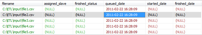
In your favourite SQL Client run following query to see the records that were inserted by the transformation:

SELECT

*

FROM

FILE_QUEUE

;

Once you inspected the results run:

DELETE FROM FILE_QUEUE ; 

The idea is that this process is scheduled to run continuously (every 10 seconds or so).

Define Slave Servers

First off, we will create a table that stores all the details about our slave servers. In your favourite SQL Client run following statement:

CREATE TABLE SLAVE_LIST

(

id INT

, name VARCHAR(100)

, hostname VARCHAR(100)

, username VARCHAR(100)

, password VARCHAR(100)

, port VARCHAR(10)

, status_url VARCHAR(255)

, last_check_date DATETIME

, last_active_date DATETIME

, max_load INT

, last_load INT

, active CHAR(1)

, response_time INT

)

;

Open the Initialize SLAVE_LIST transformation in Kettle. The transformation allows to easily configure our slave server definition. We use the Data Grid step to define all the slave details:

• id
• name
• hostname
• username
• passoword
• port
• status_url
• last_check_date: keep empty, will be populated later on
• last_active_date: keep empty, will be populated later on
• max_load
• last_load: keep empty, will be populated later on
• active
• response_time: keep empty, will be populated later on

As you can see, we use an Update step: This allows us to basically change the configuration at any time in the Data Grid step and then rerun the transformation.

Execute the transformation.

Run following statement in your favourite SQL client :

SELECT * FROM SLAVE_LIST ;

Monitor Slave Servers

Features:

• Checks the status of the active slave servers defined in the SLAVE_LIST
• Checks wether they are still active
• Calculates the load (number of active jobs) per slave server
• Calculates the response time

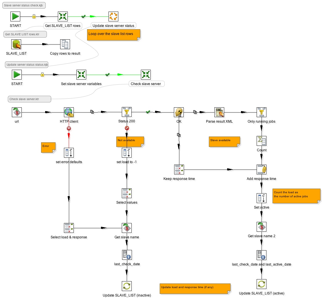
Open following files in Kettle:

• Slave server status check.kjb

• Get SLAVE_LIST rows.ktr: Retrieves the list of defined slave servers (including all details) and copies rows the to the result set
• Update slave server status.kjb: This job gets executed for each input row (=loop)

• Set slave server variables.ktr: receives each time one input row coming from the result set of Get SLAVE_LIST rows.ktr and defines variables for each field, which can be used in the next transformation
• Check slave server.ktr: 

• Checks whether the server is not available or status is 200 and then updates the SLAVE_LIST table with an inactive flag and last_check_date.
• If the server is available:

• it extracts the amount of running jobs from the xml file returned by the server
• keeps the response time
• sets an active flag
• sets the last_check_date and last_active_date (both derived from the system date) 
• updates the SLAVE_LIST table with this info

Please find below the combined screenshots of the jobs and transformation:

So let's check if all our slave servers are available: Run Slave server status check.kjb. Run the following statement in your favourite SQL client:

SELECT * FROM SLAVE_LIST;

The result set should now look like on the screenshot below, indicating that all our slave servers are active:

Distribution of the workload

So far we know the names of the files to be processed and the available servers, so the next step is to create a job that processes one file from the queue on each available slave server.

Open Process one queued file.kjb in Kettle.

This job does the following:

• It checks if there are any slave servers available that can handle more work. This takes the current and maximum specified load (the number of active jobs) into account.
• It loops over the available slave servers and processes one file on each server.
• In the case that no slave servers are available, it waits 20 seconds.

Some more details about the job steps:

• Any slave servers available?: This fires a query against our SLAVE_LIST table which will return a count of the available slave servers. If the count is bigger than 0, Select slave servers is the next step in the process.
• Select slave servers: This transformation retrieves a list of available slave servers from the SLAVE_LIST table and copies it to the result set.
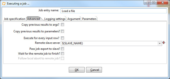
• Process a file: The important point here is that this job will be executed for each result set row (double click on the step, click on the Advanced tab and you will see that Execute for each input row is checked).

Open Process a file.kjb. 

This job does the following:

• For each input row from the previous result set, it sets the slave server variables.
• It checks if there are any files to be processed by firing a query against our FILE_QUEUE table.
• It retrieves the name of the next file that has to be processed from the FILL_QUEUE table (a SQL query with the limit set to 1) and sets the file name as a variable
• It updates the record for this file name in the FILE_QUEUE table with the start date and assigned slave name.
• The Load a file job is started on the selected slave server : Replace the dummy Javascript step in this job with your normal ETL process that populates your data warehouse. Some additional hints:

• The file name is available in the ${FILENAME} variable. It might be quite useful to store the file name in the target staging table. 
• In case the ETL process failed once before for this file, you can use this ${FILENAME} variable as well to automatically delete the corresponding record(s) from the FILE_QUEUE table and even the staging table prior to execution. 
• Note that the slave server is set in the Job Settings > Advanced tab:
  

• If the process is successful, the record in the FILE_QUEUE table gets flagged respectively. The same happens in case the process fails.

Test the whole process

Let's verify that everything is working: Open Main Job.kjb in Kettle and click the Execute icon.

Now let's see if 4 files were moved to the archive folder:

This looks good ... so let's also check if our FILE_QUEUE table has been updated correctly. Run following statement in your favourite SQL client:

Note that the last file (file5.csv) hasn't been processed. This is because we set up 4 slave servers and our job is passing 4 files to each of the slave servers. The last file will be processed with the next execution.

Pentaho Data Integration: Best practice solutions for working wit

Pentaho Data Integration: Best practice solutions for working with huge data sets

Assign enough memory

Open pan.sh and kitchen.sh (and spoon.sh if you use the GUI) in a text editor and assign as much memory as possible.

Data input

Data from a database table can only be imported as fast as the database allows it. You cannot run multiple copies of a database table input step.
Text files are more convenient, as you can copy them across servers (your cluster) and read them in simultaneously. Another really cool feature that Kettle has is that you can read in text files in parallel (check the "Run in parallel" option in the step configuration and specify the number of copies to start with in the step context menu). How does this work? If your file has a size of 4 GB and you specified 4 copies of the text step, each step will read in chunks of that file at the same time (to be more precise: the first copy will start reading at the beginning of the file, the second copy will start at the first line that is found after 1 GB, the third copy will start at the first line that is found after 2 GB and so on).

Run multiple step copies (Scale up)

Find out first how many cores your server has, as it doesn’t make sense assigning more copies than there are cores available.
Linux: cat /proc/cpuinfo
Have a look how many times processor is mentioned. The first processor has the id 0.

Make sure you test your transformations first! You might get unexpected results (see my other blog post for more details).

Usually you should get better performance by specifying the same amount of copies for steps where possible (herewith you create dedicated data pipelines and Kettle doesn’t have to do the work of sending the rows in a round robin fashion to the other step copies).

Run a cluster (Scale out)

You can run your ETL job on multiple slave servers. Kettle allows you to specify a cluster via the GUI. For this to work, you have to set up Carte first, which comes with PDI (see my other blog post for details).
Of course, you can combine scale out and scale up methods.

Adjust Sort Rows step

Make sure you set a proper limit for Sort size (rows in memory) and/or maybe as well Free memory Threshold (in %).

You can run the Sort Rows step in multiple copies, but make sure you add a Sorted Merge step after it. This one will combine and sort the results in a streaming fashion.

Use UDJC instead of Javascript

Java code will execute faster than javascript, hence use the User Definied Java Class step instead of the Javascript step where possible.

Pentaho Metadata Editor: Joining two fact tables

Pentaho Metadata Model: Joining two fact tables

This tutorial was possible with the help of Will Gorman, Vice President of Engineering at Pentaho

The data

Metadata Model

My Suggestions

Tutorial Details

• Software: PME 3.7 (download here), a database of your liking, in example MySQL
• Knowledge: Intermediate (To follow this tutorial you should have good knowledge of the software and hence not every single step will be described)
• Tutorial files can be downloaded here

The Pentaho Metadata layer is amazing: It allows end users to build reports without actually writing a line of SQL. Database and/or table changes can be easily accommodated by only changing the references in the metadata model and hence reports, dashboards, etc stay unaffected. 

While it is fairly easy to set up a metadata model with one fact table (and some dimensions), using more than one fact table (which also might have different granularity) posses a challenge for many users. Is it really possible to do this in PME (Pentaho Metadata Editor)? The answer is yes, although in the current version I don't consider it to be an ideal solution and I hope that in future it will be possible to visually design this in the relationship diagram. 

In this session I'd like to discuss the approach of integrating more than one fact table into your metadata model. 

The data

We will base our example on this simple schema:

CREATE SCHEMA 

metadatatest

;

CREATE TABLE

metadatatest.fact_sales

(

date_id INT(255),

location VARCHAR(70),

sales INT(255)

)

;

INSERT INTO 

metadatatest.fact_sales 

VALUES

(1,"London", 34),(1,"Manchester", 44),(2,"London",24),(2,"Manchester",35),(2,"Bristol",34),(3,"London",53)

;

CREATE TABLE

metadatatest.fact_stock

(

date_id INT(255),

location VARCHAR(70),

aisle VARCHAR(70),

stock INT(255)

)

;

INSERT INTO 

metadatatest.fact_stock

VALUES

(1,"London","aisle 1", 34),(1,"London","aisle 2", 44),(1,"London","aisle 3", 234),(1,"Manchester","aisle 1", 44),(1,"Manchester","aisle 2", 344),(2,"London","aisle 1",24),(2,"London","aisle 2",25),(2,"Manchester","aisle 1",35),(2,"Bristol","aisle 1",34),(2,"Bristol","aisle 2",324),(3,"London","aisle 1",53)

;

CREATE TABLE

metadatatest.dim_date

(

date_id INT(255),

date DATE

)

;

INSERT INTO

metadatatest.dim_date

VALUES

(1,"2011-01-01"),(2,"2011-01-02"),(3,"2011-01-03")

;

What we want to achieve is basically getting the same result out of PME as with following summary query:

SELECT

*

FROM

(

SELECT

date,

SUM(sales) AS sales

FROM

metadatatest.fact_sales s

INNER JOIN

metadatatest.dim_date d

ON

s.date_id=d.date_id

GROUP BY 1

) a

INNER JOIN

(

SELECT

date,

SUM(stock) AS stock

FROM

metadatatest.fact_stock s

INNER JOIN

metadatatest.dim_date d

ON

s.date_id=d.date_id

GROUP BY 1

) b

ON

a.date=b.date

;

Open your favourite SQL client and run these queries.

The aggregation query gives back following result:

Metadata Model

So let's start creating our Metadata model: One thing to keep in mind is that our two fact tables have different granularity. In PME you cannot just import them as physical tables, then place them both in a business model and create a relationship between them: Such a model will not return correct aggregations.

The critical element is: You basically have to specify the "physical tables" as join of your star schemas. What I mean by this is that you write a query that joins your fact table with all the dimension tables. This query returns a result set which can act as a "physical table" in PME (although the wording "physical table" doesn't make sense in the context, it is more a derived table or better said a view). 

In our case we will have two derived tables. These two derived tables have to have the same granularity:

• Sales Table: a join of the fact_sales table with the date dimension
• Stock Table: a jon of the fact_stock table with the date dimension, aggregated by date and location

  

1. Open PME and create a new domain.
2. Set up your database connection to the just created schema.
3. Reference our two fact tables.
4. Double click on the fact_sales table. The properties window will be shown.
5. Click on the green plus icon in the Properties section and add the Target Table property. Click OK.
6. Fill out the Target Table field with this query:
    
   SELECT date date_1, location location_1, SUM(sales) AS sales FROM metadatatest.fact_sales s INNER JOIN metadatatest.dim_date d ON s.date_id=d.date_id GROUP BY 1, 2).
   Note we gave the date and location columns intentionally different names so that they are later on easier to distinguish from the other fact table's fields.
   
7. Click OK to close the Properties window.
8. Double click on the fact_stock table. The properties dialog will be shown.
9. Click on the green plus icon and add the Target Table property. Click OK.
10. Fill out the Target Table field with this query: Fill out the Target Table field with this query:
    SELECT date, location, SUM(stock) AS stock FROM metadatatest.fact_stock s INNER JOIN metadatatest.dim_date d ON s.date_id=d.date_id GROUP BY 1, 2
    
11. Click OK to close the Properties window.
12. Create a business model and drag and drop the physical tables into the Business Tables folder. Your Tables should now look like this (as you can see they have same granularity now):
    
    
13. Next create the relationship: Drag and drop the business tables onto the canvas, hold down the CTRL key, mark the first table and then the second one and right click. Choose Add Relationship ...
14. Set Relationship to N:N and Join type to Inner. 
15. Tick Complex Join? and copy following lines into the Complex Join Expression: 
    AND([BT_FACT_SALES_FACT_SALES.BC_FACT_SALES_DATE_1]=[BT_FACT_STOCK_FACT_STOCK.BC_FACT_STOCK_DATE]; [BT_FACT_SALES_FACT_SALES.BC_FACT_SALES_LOCATION_1]=[BT_FACT_STOCK_FACT_STOCK.BC_FACT_STOCK_LOCATION])
    
    
    
16. Click OK.
17. Save the model. Now we are ready to test if it is working properly.
18. Click on the Query Editor icon. Select Date, Sales and Stock as columns, then press the Play button. Examine the result: It returns exactly the same values as the SQL query we ran at the beginning of the tutorial. If you are curious you can as well click on the SQL icon and you can see which SQL query PME created under the hood.
    
    
    

My Suggestions

It is important to provide feedback to the developers of such great products as the PME. I can see in my daily work what a big impact this product makes. I can see end users who can finally create reports to their liking without running to a report designer and waiting for the result to be delivered. When you create a lot of reports you don't have to worry if a database change results in having to change all the references in all your reports. From my point of view a metadata model is a key element in a BI system. 

In the beginning of this article I already mentioned that I don't think the current way of setting up this solution is ideal. The reason for this is that it breaks the concept. Normally you would define the relationships between tables in a business model and the SQL would be automatically created. When dealing with more than one fact table (with different granularity), you have to use a completely different approach and write a SQL query yourself by joining your fact table all dimension tables and only then you can create the relationship diagram.

It's not a problem of "Oh I have to write a query", but it is more a problem of consistent approach. I'd really welcome if we could design the complete model in a relationship diagram (consistant approach) instead of hacking the shortcomings by providing SQL queries. I think the user experience would be much better.

I set up a JIRA case on the Pentaho website to, please show your support by voting for it and we might see this feature implemented soon!

At the end of the session I'd like the thank Will for his great support!